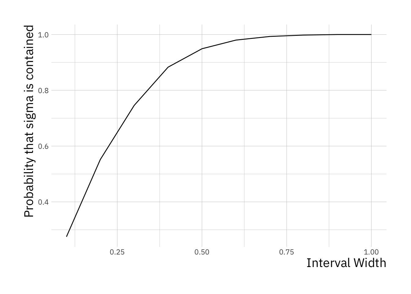
# create a vector to store the number of times
# the population variance is contained
sigma_contained <- rep(0, n_interval_widths)

for (replicate in 1:nreps) {

  x <- rnorm(n, mean = mu, sd = sigma) # simulate a data set

  sigmabar <- sd(x) # compute the sample standard deviation

  # for each interval width that we are testing ...
  for (j in 1:n_interval_widths) {
    # check if the interval contains the true mean
    if ((sigma > sigmabar - 0.5 * interval_width[j]) &
        (sigma < sigmabar + 0.5 * interval_width[j])) {

      # if it is, we increment the count by one for this width
      sigma_contained[j] <- sigma_contained[j] + 1
    }
  }
}

probability_var_contained <- sigma_contained / nreps

# create a data frame containing the variables we wish to plot
df <- data.frame(interval_width = interval_width,
        probability_var_contained = probability_var_contained)

# initialise the ggplot
plt <- ggplot(df, aes(x = interval_width, y = probability_var_contained))
# create a line plot
plt <- plt + geom_line()
# add a horizontal axis label
plt <- plt + xlab("Interval Width")
# create a vertical axis label
plt <- plt + ylab("Probability that sigma is contained")

# plot to screen
print(plt)
